Generate Word Clouds in R from Conference Tweets
#SACConf and #motorspeech18
It’s been just about a week since the Speech-Language and Audiology Canada (SAC) Conference. Clinical researchers in speech-pathology and audiology from all across Canada came to take part in three days of talks, poster presentations, product demos, and planning meetings. Because the conference is so large, there tend to be several overlapping sessions at once. There’s pretty much something there for everyone, but there’s also a good chance that you’ll be torn between attending two sessions that overlap and have to choose one. Fortunately, the SLP crowd is a twitterful bunch, and are quick to update other SLPeeps near and far on professional tidbits they find of interest.
Cool story. But I’m just here for the word cloud… bring me to the word cloud.
I am admittedly a novice tweeter/twitterer/person who uses twitter. There’s a lot of pressure to be clever and impactful in 140 (nay, now 280) characters. My fear of misconjugating the verb “to tweet” also may have some bearing on my reluctance. This is not a baseless fear; an unfortunate incident in my early twitter days led me to accidentally calling a dear friend a terrible name in a poor attempt at the past tense. Still unsure TBH 🤷♀ but I have learned I am not entirely alone.1
Reluctantly, I have taken another stab at it this past year, prompted by needing to familiarize myself with it for R-Ladies. All the cool girls have it and it is a quasi-requisite for being fully connected with the community. I have since realized though (and actual twitter die-hards could tell you they’ve been saying this for years) it turns out to be a great toy/tool to stay connected with the academic community, as well as within the clinical SLP world. Many journals tweet out recently published articles. Researchers have lengthy debates and exchanges of ideas. Clinicians post queries, findings, and blogs. And, the topic relevant to this particular post, academic conference attendees can document their experiences to the great wide interwebs with the use of conference hashtags.
Goal: Generate a word cloud from #SACConf tweets
A few considerations to bear in mind before forging ahead:
- While there are many fun text-based analyses one can do with twitter scraping, I know very little to absolutely nothing about that. If you’re into that though, check out the many blog posts that have referenced
rtweetto see what people have come up with. - There are apps in existence that will execute this goal for you, but that is besides the point.
- There used to be a nifty way to compile tweets using Storify, but this won’t be possible after May 16, 2018. Fortunately, Maëlle Salmon wrote an equally nifty post on how to do just that using
rtweet.
Calling all hashtagged tweets
Assuming there’s an agreed-upon communal hashtag for a given conference, this is a fairly quick and painless fun little task. In the case of the SAC Conference, the hashtag stays the same year to year: #SACConf. If, however, something like #MSC16 turns out not to be the 2016 Motor Speech Conference and instead is flooded with tweets from the Manufacturing Supply Chain annual meeting, things can get hairy (as was once narrowly avoided at what became #motorspeech16). It also helps if several distinct voices are tweeting about the same thing.
Accessing tweets
In this case we’re looking at a finite number of tweets tagged with #SACConf (not case sensitive), so we’re interested in collecting all of them. You could also specifiy a maximum number and/or whether you want recent or popular tweets. A couple of days after the conference had ended, this is what I entered:
library(rtweet)
library(knitr)

tweets <- search_tweets("#sacconf", lang="en",include_rts = FALSE)
head(tweets$text)
## NULLTiming is crucial here if you’re chasing hashtags, though, so be cautious.
Gotta act fast!
Sadly/unsurprisingly, Twitter Co. is a clever money-making machine and doesn’t actually let you access old Twitter API queries without a cost (either financially or through a lot of hacking). That is, you can access recent tweets for free, but you gotta pay up if you want to access tweets earlier than the last week or so. You can purchase the option to go back in time, but given I stopped even getting guacamole on my burritos when the price went up a whopping 87 cents there was absolutely zero chance of that happening for me. You are limited to NINE DAYS of queries so you’ve got to be quick! By the time this post actually makes it to the web, I can almost guarantee that it will have been more than 9 days from the critical start time that I wanted the tweets from, so FEAR NOT - there is some hope for the lazy like me… sort of. If you know the critical 9-day period for your tweets of interest is closing in, you can do a quick scrape, save the results to an .RData file, and load that in to analyze/wordcloudize later.
# Save tweets for later (and note when saved):
save(tweets, file="sacconf_tweets.RData")

# And access them later at will...
# load("sacconf_tweets.RData")
Note that if you go this route, you don’t have to use search_tweets again (and in fact if you do and you’re past the 9 day window you’ll get a very different sample/nothing).
If you miss that 9-day window though, tough cookies if you wanted tweets from a general query. If you’re only interested in particular individuals’ tweets, however, you’re in luck: you can access a single twitterer’s entire timeline without restriction (so, for example, one could pull all the tweets from @wespeechies at any time).
When was the action happening?
Now that we’ve got our tweets, we can see when most of the tweeting action was happening by plotting the density of the time stamp of the post (the created_at variable). This can help confirm that you’ve got the right timeframe and that the tweet schedules matches your expectations for that time frame. There were 131 tweets in total during the time period I queried.
library(ggplot2)

ggplot(tweets, aes(created_at))+
     geom_density(alpha=.75, fill="#4CABDA")+ # fill with main SAC logo blue
     ggtitle("#SACConf Tweets")+
     ylab("Density")+
     xlab("Time of tweet")+
     theme(panel.background = element_rect(fill="#96AAB5"),
           title = element_text(color="#F09240", size=20)) # background and text colour also from SAC Conference logo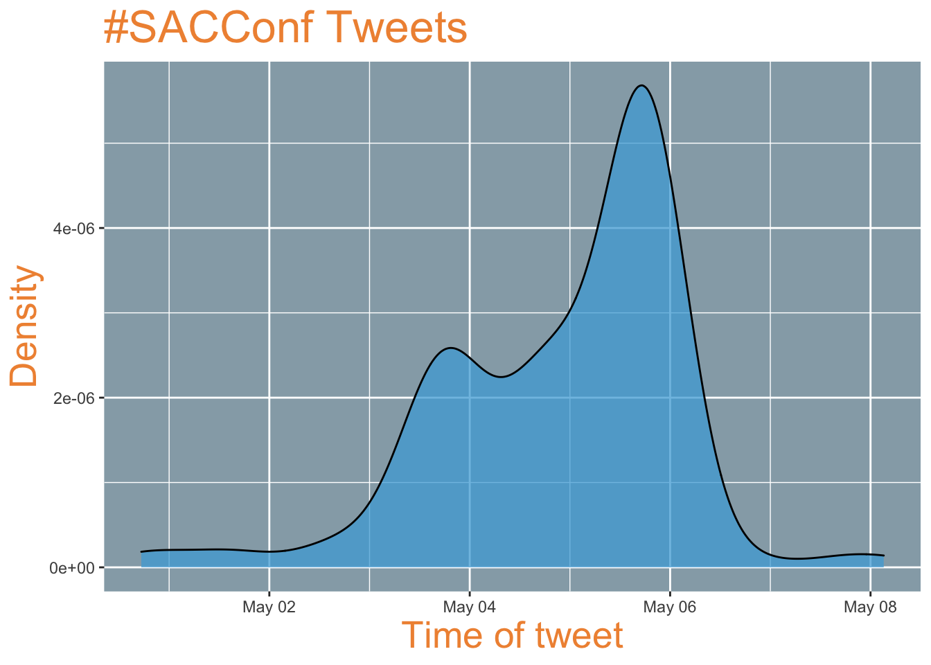
There’s a peak at the end of the first day of talks (May 3) and a flurry of activity at the end of the conference.
Making the word cloud
Tidying the word list
Now we have to check to make sure the top appearing words are relevant and informative. For the sake of language, I do love my function words, but the appearance of “the” and “a” in a word cloud does little to conjure up the spirit of the tweets. We’ll first eliminate basic function words using the stopwords corpus from the rcorpora package (thanks again Maëlle for the how-to).
library(rcorpora)
library(tidytext)
library(dplyr)

stopwords <- corpora("words/stopwords/en")$stopWords
tweets_words <- tweets %>%
     unnest_tokens(word, text) %>%
     count(word, sort=TRUE) %>%
     filter(!word %in% stopwords)
Looking at just the top ten words gives some indication that there may still be strings we don’t want. “https” and “t.co” for instance don’t make the cut. “sacconf” understandably occurs much more frequently than the other words (it appears in every tweet because it was the search term), but we’ll deal with that in a minute.
ggplot(head(tweets_words, n=10), aes(x=reorder(word, -n), y=n))+
     geom_bar(stat="identity")+
     ggtitle("Top 10 words in #SACConf tweets: First pass")+
     theme(axis.text=element_text(size=14, angle = 90, face="bold"), axis.title.x = element_blank(), title = element_text(size=14))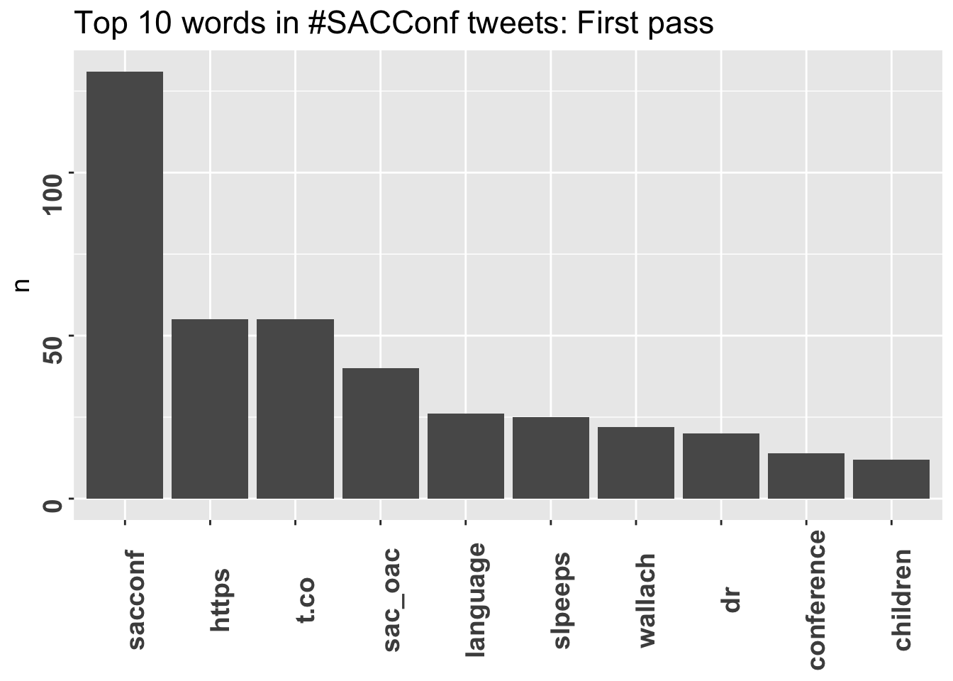
After looking at the top 100 words, I’ve made a few additional cuts. I debated cutting people’s names but have left them in for now - there are certain names that received substantial attention and it’s informative to leave them in.
# Remove some more uninformative words

tweets_words <- tweets_words %>%
     filter(!word %in% c("t.co", "https", "00", "1", "2", "3", "4", "5", "9", "p.m", "download", "rt", "gt", "dr"))
Customizing your cloud
When I originally sat down to do this, I planned on using the wordcloud package because a) it seemed pretty relevant and b) I found this handy tutorial on another blog. After a bit of digging and playing around though, I decided to go with wordcloud2 because it had a few more fun features to exploit.
All you really need to generate a word cloud at this point is
`wordcloud2(data = tweets_words)but I’ve made a few extra tweaks in the version below. Word size, unless otherwise specified, is dictated by the number of occurrences. Since the entry “sacconf” appears once for every tweet (since it was the word used to scrape the tweets in the first place), it shows up waaaaay more often than all the other words. I want to keep it in, but don’t want it dominating the scene quite so much, so I’ll resize it. I’ll also change the colour scheme to match the SAC Conference logo, add a black background, set the rotation of the words, and filter out words that appear less than five times.
Word cloud! At last!
library(wordcloud2)

tweets_words$n[tweets_words$word=="sacconf"] <- 70

wordcloud2(data = tweets_words, backgroundColor = "black",color = rep_len(c("#96AAB5", "#F09240", "#3C89AE", "#4EA9A4", "#4CABDA"), nrow(tweets_words)), minRotation = -pi/6, minSize=5, size=1)
Bonus! #motorspeech18
I also logged tweets after the Motor Speech Conference this February. There are admittedly fewer motor speechies in the twittersphere (solid shout out to Tricia McCabe for expertly holding down the fort as the rest of us tried to keep up). While there was a higher tweets-to-tweeter than for #SACConf, I think the end result still winds up being fairly representative and a fun contrast. No code displayed here, but basically the same setup2.

C’est tout! A fun little exercise in visualizing the most popular words used to tweet out sound bites from a conference. This would be easily generalizable to other twitter trends of interest, just bearing in mind that you either need to a) keep in mind the 9 day limit or b) choose one (or a subset of) individuals to scrape tweets from.
This riveting press conference clip of Twitter’s co-founder responding to the question “Are you a Twitterer or a Tweeter” clarifies nothing, but does make me feel a bit better as even he doesn’t know how to conjugate it. Sure this was nearly a decade ago, but that’s besides the point. ↩︎
I removed names this time, since they often only appeared once or twice, and I didn’t restrict it to low frequency words otherwise. Color scheme is FantasticFox1 from the Wes Anderson films palettes for no reason other than I liked the way it looked and it is a fantastic, if totally unrelated, film.↩︎